Generate and inspect magnetic field and current density plots

Before starting

Field plots help inspect how a model distributes a selected electromagnetic quantity in space. They supplement the extracted circuit result; the colour plot alone does not establish convergence or physical accuracy. This worked example requests magnetic flux density B on a plane above the strip and current density J on the conductors.

Download the complete field-example ZIP or save the three complete files below together in a new writable folder. Use matching licensed InductEx®/TTH tools. The recorded CLI is InductEx® 8.0.1 with TTH 1.1.50, and the native controls were exercised in the current Windows source candidate. This teaching process is not a calibrated fabrication stack.

Define the field request and sampling plane

Plot [B, J] belongs inside the IXI COMMAND record. FPLANE is outside STRUCT: its corner and translation coordinates are in metres even though the process uses Units = 1e-6. The supplied plane runs from x = -5 to 105 micrometres and y = -10 to 20 micrometres, translated to z = 2 micrometres. Keep each coordinate triple on its own line.

FieldMeshSize = 5 uses the process length unit and controls this plane sampling. SegmentSize = 2 still controls the cuboid conductor mesh. Changing field sampling, changing the conductor mesh and changing arrow density are different operations. The checked generated request applies the plane to B; J is written on conductor geometry, not on the B sampling plane.

Generate and open the current output

1. Open strip.ixi in Studio, save the complete inputs and use the normal extraction action. For the optional CLI route, run the command below from the folder containing all three files.
2. Check the current completion verdict and diagnostics. This example generates output/B_strip.vtk and output/J_strip.vtk, along with the model mesh and numerical results. The unchanged extracted L1 remains 3.89648e-12 H at GUI precision.
3. Open B_strip.vtk through File > Open or the project artifacts. In Fields, select the required array and choose Apply field view. Keep the full array name visible when recording or comparing a view.
4. The checked files contain 10.000GHz_p1_imag and 10.000GHz_p2_imag. Next array selects the other excitation and wraps back. These are the arrays actually emitted by this run; do not assume that every requested file contains both real and imaginary arrays.

inductex strip.ixi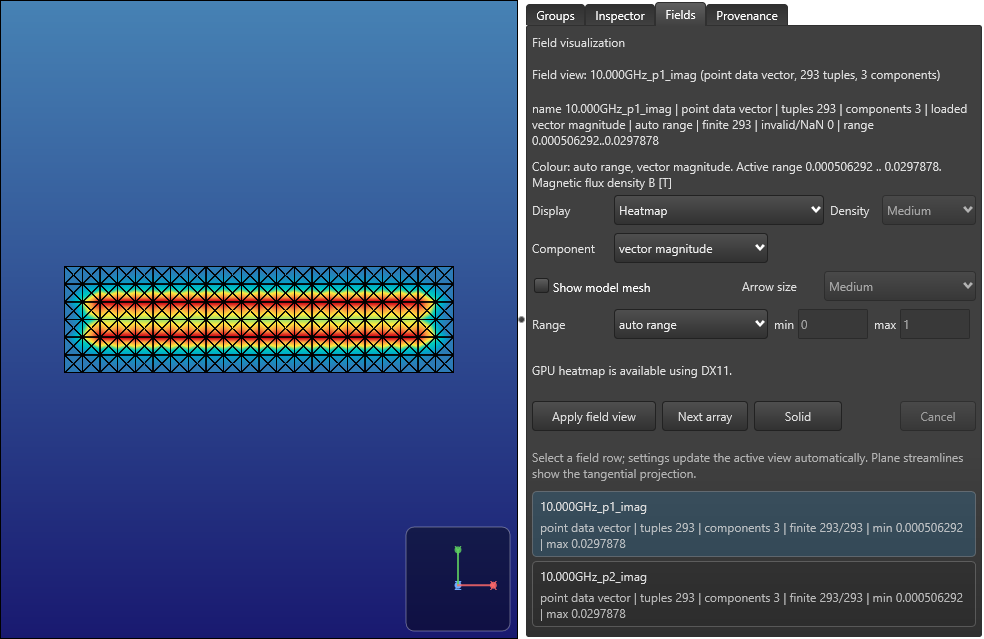

Choose the quantity and display

Use Component to choose vector magnitude or a signed X, Y or Z component. The checked Z component crosses zero; its colour range has both negative and positive values. Magnitude is computed from the selected real or imaginary vector array. It is not the combined complex AC amplitude and is not a time animation.

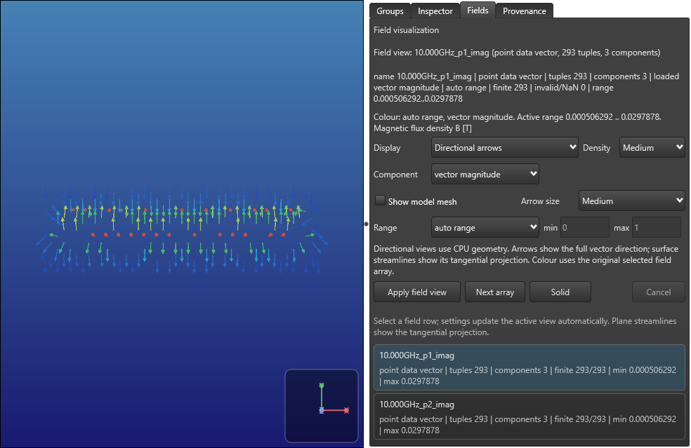
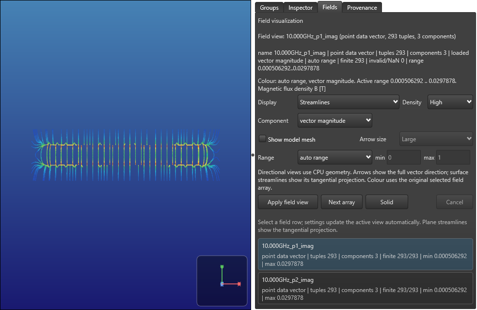
Heatmap colours the selected quantity on the supplied geometry. Directional arrows show the full vector direction, while streamlines on a plane follow its tangential projection. A vector normal to the plane can therefore have arrows without an in-plane streamline. These traces describe sampled spatial data, not moving particles or an additional field solve.

Density and Arrow size control readability. In the checked view, Low, Medium and High density increased generated arrow geometry while the B array retained the same 293 tuples. A larger arrow size changed the display extent without changing its tuple count. Increasing those settings does not refine the solver mesh or add field samples.

Set a useful range and recover an invalid value

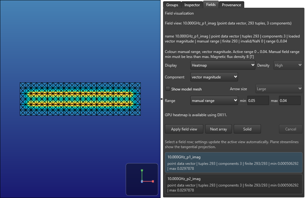
Auto range uses the selected data. For a controlled comparison, use the same quantity/component and explicit manual endpoints in both views; independently auto-ranging two plots can make unlike magnitudes look similar. For this B magnitude, 0 to 0.04 T is a valid illustrative manual range. It is a display choice, not an accuracy tolerance.

Manual endpoints must be finite and minimum must be less than maximum. The checked change from minimum 0 to 0.05, while maximum remained 0.04, produced a diagnostic and retained the last valid 0 to 0.04 payload. Correcting minimum to 0 recovered the manual view; choosing auto range recovered its original data-derived endpoints. Read the active range and message rather than assuming that every typed value was applied. The exact diagnostic is: Manual field range min must be less than max.

Keep field and model coordinate scales consistent

Leave Show model mesh off for this checked example. Enabling it appends the adjacent strip.msh to the metre-valued field geometry without a compatible scale conversion in the current candidate (KB-GUI-010). The combined payload width becomes about 110 instead of 0.00011, so this overlay is not accepted as an aligned model context.

Disabling the option restores the field-only bounds and range. Keep the original output files; do not rewrite their coordinates merely to obtain a plausible picture. The candidate needs a validated coordinate-system relationship before the grey model context can be relied on for this route. A nearby filename alone does not establish equal units.

Inspect current density and save the view

Open J_strip.vtk and apply the intended array in Fields. The checked J file contains 14301 finite three-component tuples for each of its two excitation arrays. This is conductor current density output, with generated J units of A/m2; it is distinct from the B plane.

Use Solid to return to ordinary geometry and Apply field view to restore the selected field. The checked route recovered the same B array, range and bounds after this change. Export snapshot writes the current field canvas and a companion report; review the report for private paths before sharing it. The dedicated snapshot guide explains save cancellation and failure/retry.

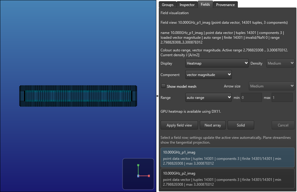
Check output identity before interpreting values

Keep the saved request, solver version, generated filename, complete array name, quantity and coordinate scale together. The checked B VTK has a misleading free-text title saying Electric current density generated by TTH (KB-OUTPUT-001). Its generated request explicitly routes B to B_strip.vtk, and Studio labels that known filename as B in Tesla. Neither a generic title nor a renamed file prefix is sufficient authority for an arbitrary output.

The CLI and native runs emitted identical parsed vector arrays. Studio magnitude and signed-component endpoints agreed with those values within the stated binary32 display-representation allowance. This checks data/display consistency, not an independent physical field reference or convergence criterion.

If a file is missing, start with the current run diagnostic, requested Plot values and the supported mode/engine. If the view seems empty, check the selected array, component, range and model-overlay state before changing the physical calculation. Cancellation, field-view state after restart, other VTK formats and final distributed-package acceptance still require their own checks.

Complete strip.ixi

* Parameterised inline equivalent of the maintained microstrip geometry
$COMMAND
  MeshFile "strip.msh"
  MeshType CUBE
  Mode MQS
  Plot [B, J]
  Netlist "strip.cir"
  Process "process.ldf"
$END
$VARIABLE
  Name strip_length
  Value 100
$END
$VARIABLE
  Name strip_width
  Value 10
$END
$STRUCT
  Name inline_strip
  $POLY
    Layer M1
    XY
    (0,0)
    (0,%strip_width)
    (%strip_length,%strip_width)
    (%strip_length,0)
    (0,0)
  $END
  $PATH
    Layer TERM
    Width 1
    XY
    (0,%strip_width)
    (0,0)
  $END
  $PATH
    Layer TERM
    Width 1
    XY
    (%strip_length,%strip_width)
    (%strip_length,0)
  $END
  $TEXT
    Text "P1 M1 M0"
    Layer TEXT
    XY
    (0,%strip_width/2)
  $END
  $TEXT
    Text "P2 M1 M0"
    Layer TEXT
    XY
    (%strip_length,%strip_width/2)
  $END
$END

$FPLANE
  Coords
  (-5e-6,-10e-6,0)
  (105e-6,20e-6,0)
  Translate
  (0,0,2e-6)
$END

Complete process.ldf

* Public microstrip teaching stack; dimensions use Units below
$Parameters
  Units = 1e-6
  SegmentSize = 2.0
  FieldMeshSize = 5.0
  AbsMin = 0.025
  GPOverhang = 5.0
  ProcessHasGroundPlane = TRUE
  GPLayer = 17
  TermLayer = 19
  TextLayer = 18
  HFilaments = 1
  TerminalInRange = 1.0
  UnitL = 1
$End
$Layer
  Number = 17
  Name = M0
  Thickness = 0.2
  Lambda = 0.09
  Order = 0
  Mask = -1
  Filmtype = S
  HFilaments = 2
$End
$Layer
  Number = 2
  Name = I0
  Thickness = 0.15
  Order = 1
  Mask = -1
  Filmtype = I
$End
$Layer
  Number = 5
  Name = M1
  Thickness = 0.25
  Lambda = 0.09
  Order = 2
  Mask = 1
  Filmtype = S
  HFilaments = 3
$End

Complete strip.cir

* Extraction topology, design inductance in henries because UnitL=1
L1 1 2 3.9e-12
P1 1 0
P2 2 0
.end