
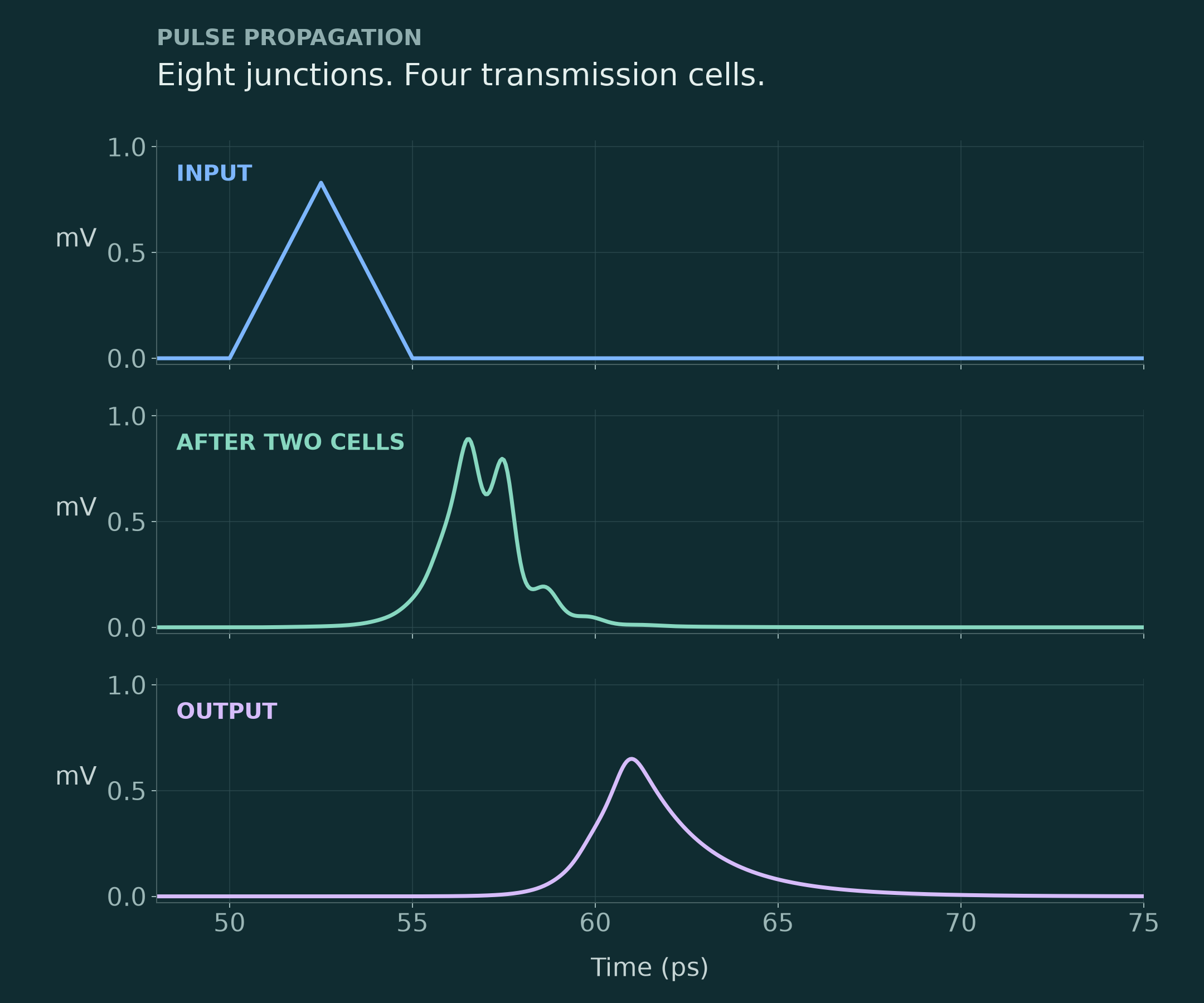
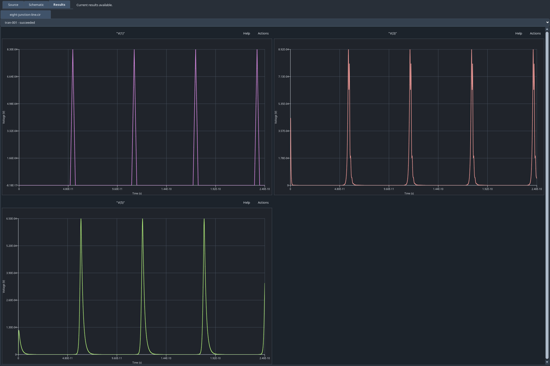
Input, midpoint and output voltages from a JoSIM®-Pro simulation of a four-cell circuit containing eight Josephson junctions.
Simulation of superconducting circuit dynamics.
JoSIM®-Pro simulates superconducting circuits as connected systems, including Josephson junctions, bias networks, transmission lines and loads. Its workspace connects the SPICE-style source with the circuit hierarchy and simulated time-domain response, so you can follow how the circuit definition leads to the resulting waveforms.
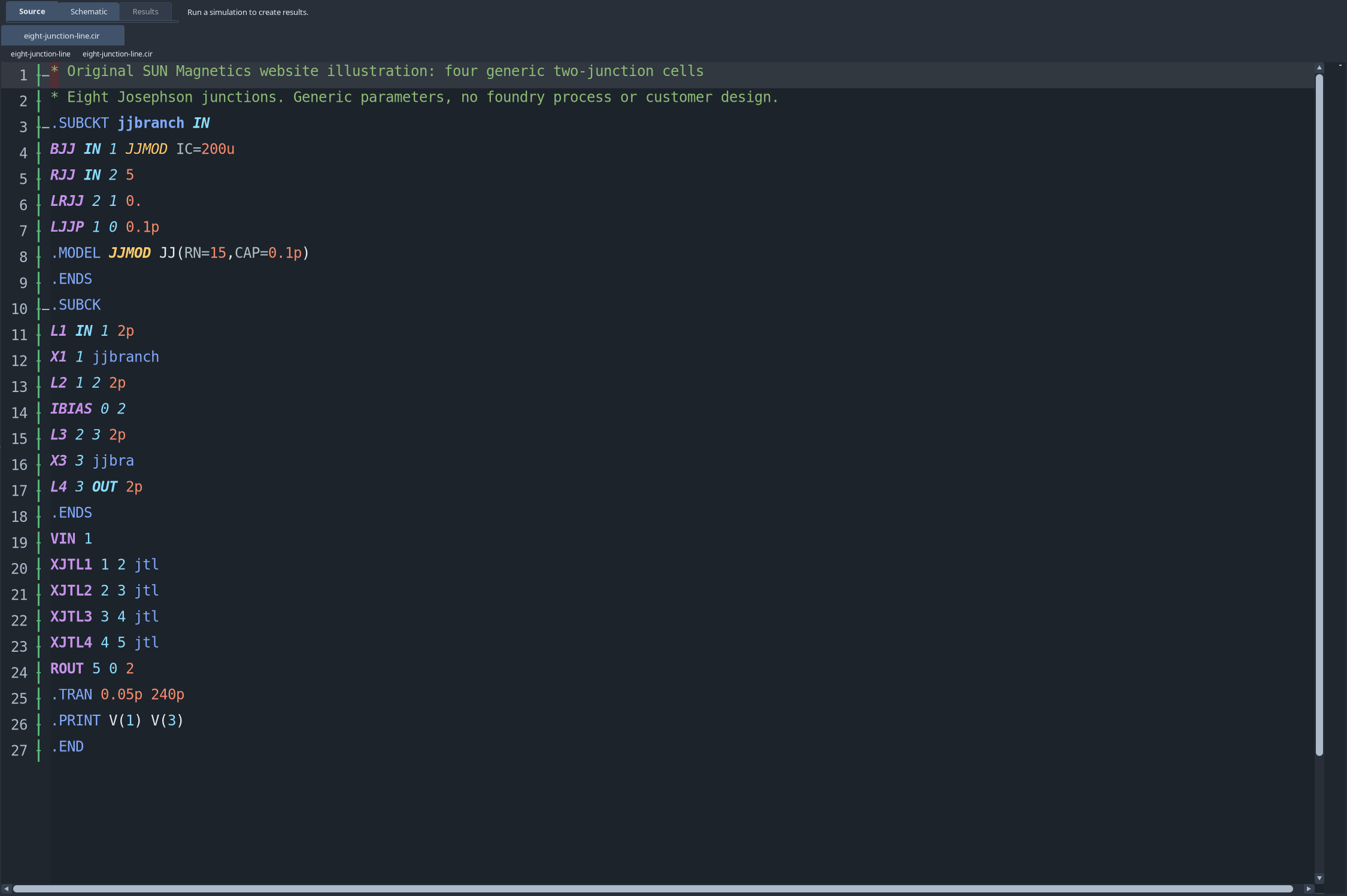
The source defines four instances of a two-junction cell, together with the bias, input source and requested voltage outputs.
Building circuits from reusable cells.
A reusable cell keeps its junction models, sources and connections in one subcircuit definition. You can then connect instances of that cell to form a larger circuit while retaining an explicit hierarchy.
In this example, four instances of a two-junction cell form a propagation path. A single input pulse passes through eight junctions before reaching the load. The source records the bias, input and requested outputs needed to reproduce the run.
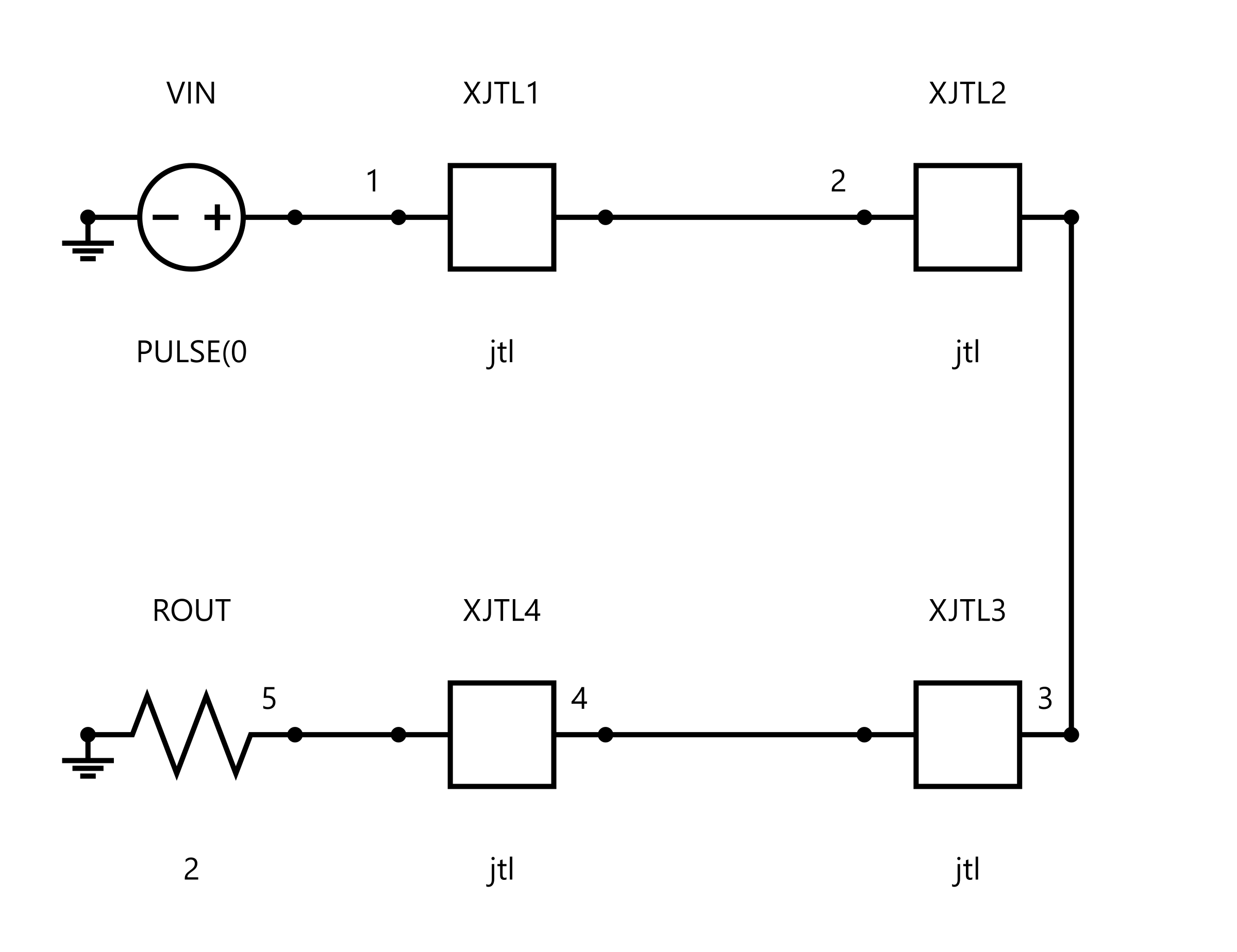
Four connected two-junction JTL subcircuits in the native schematic export. Each block represents a cell in the netlist hierarchy.
Inspecting the circuit hierarchy.
The schematic helps you check how the source definitions form the circuit before interpreting the waveforms. Here, four JTL subcircuits make up one signal path.
Each block represents a two-junction cell. Keeping the repeated stages as subcircuits makes their relationship clear without flattening the entire design into one drawing.
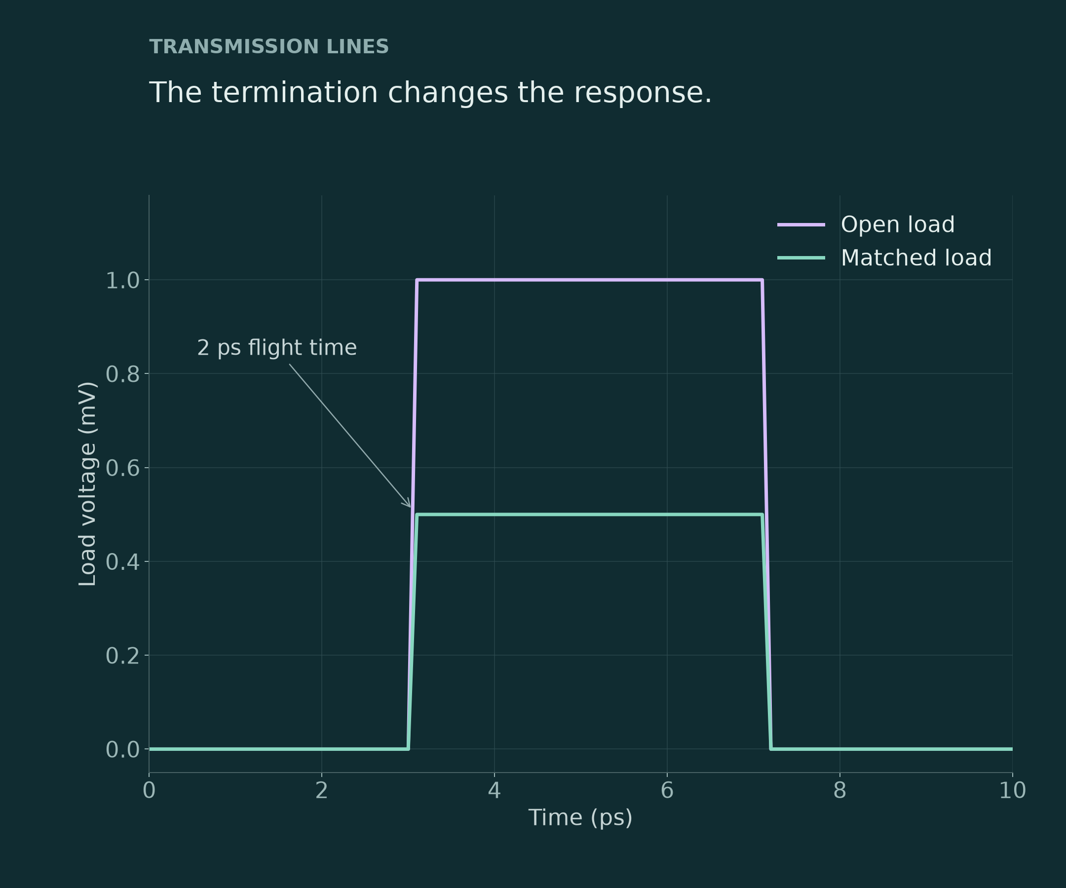
Simulated responses of matched and open loads on a lossless line with 4 Ω characteristic impedance and 2 ps flight time.
Comparing transmission-line terminations.
The interconnect and load affect the signal that reaches the end of a circuit. This lossless-line example compares matched and open terminations using a 4 Ω source, a 4 Ω characteristic impedance and a 2 ps flight time.
The simulated load plateau is 0.5 mV for the matched load and 1 mV for the open load. Comparing the traces on the same time axis shows the consequence of the termination choice within this generic model; these are simulated responses rather than measured device data.
Preparing plots and exporting results.
Plot Export Studio lets you preview selected traces and their presentation settings before exporting a figure. The demonstrated run was exported as CSV, a plot image and a schematic SVG; CSV/TSV result import is also documented for later inspection in the GUI.
Keep the source circuit, run settings and raw data with the figure so another engineer can relate the reported result to the simulation that produced it.
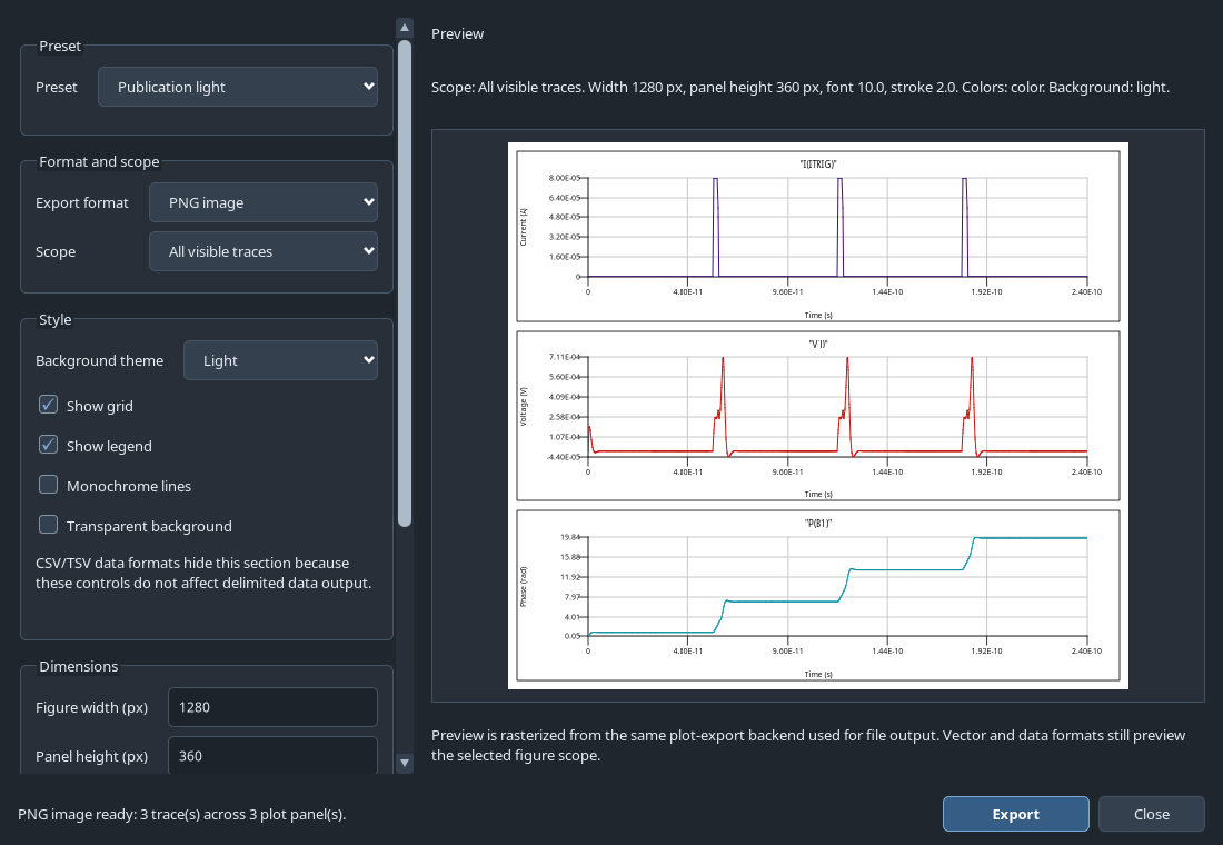
Plot Export Studio preview of the shunted-junction example, using data from the reference run.
Following a circuit through JoSIM®-Pro.
This 72-second silent tour follows the shunted-junction example through Source, Schematic, Results and export. It is composed from native interface views rather than live mouse footage. The guide below explains the same sequence.
00–09s · Three triggers and three phase slips
The example is a current-driven, resistively shunted Josephson junction, described by a classical RCSJ model.
09–18s · Define the circuit explicitly
The model specifies a 100 µA critical current, 100 fF capacitance and a separate 5 Ω shunt. The critical current is explicit, without unintended instance-area scaling.
18–27s · Inspect the circuit topology
A 70 µA bias and an 80 µA trigger briefly raise the applied current above the 100 µA critical current.
27–36s · Run and inspect the transient
The licensed GUI run produced 4,801 samples per trace.
36–45s · Relate voltage to phase
Each trigger produces one 2π phase advance. The analysis figure uses the corresponding native CSV export.
45–54s · Check one switching event
Each voltage pulse integrates to one flux quantum. The example was checked using the Josephson voltage relation, a smaller time step and an independent RCSJ reference.
54–63s · Choose traces and export
Plot Export Studio previews the selected result. The run was exported as CSV, a plot image and schematic SVG.
63–72s · Explore the circuit behaviour
Compare the source, schematic and results. The generic parameters illustrate a classical shunted junction; they do not represent a foundry-qualified device.
Automating simulation and parameter studies.
The command-line simulator provides a route for scripted runs and result-file output. For example, josim-pro-cli -o results.csv circuit.cir runs a circuit and writes its results. Retain the input, options, software version and licence context when checking reproducibility.
Optimum™
Optimum™ is a separate TOML-driven command-line companion, invoked with optimum-cli configuration.toml. Its documented modes are verify, margin, yield and optimize. These check a nominal specification, explore parameter margins, estimate a model-based pass fraction and search parameter values.
Define the circuit and specification, run Optimum™ in a terminal, then inspect the generated files. The GUI shown here is the simulator workspace. The earlier Optimum™ exercise checked file handoff and a nominal specification; it did not validate manufacturing yield.
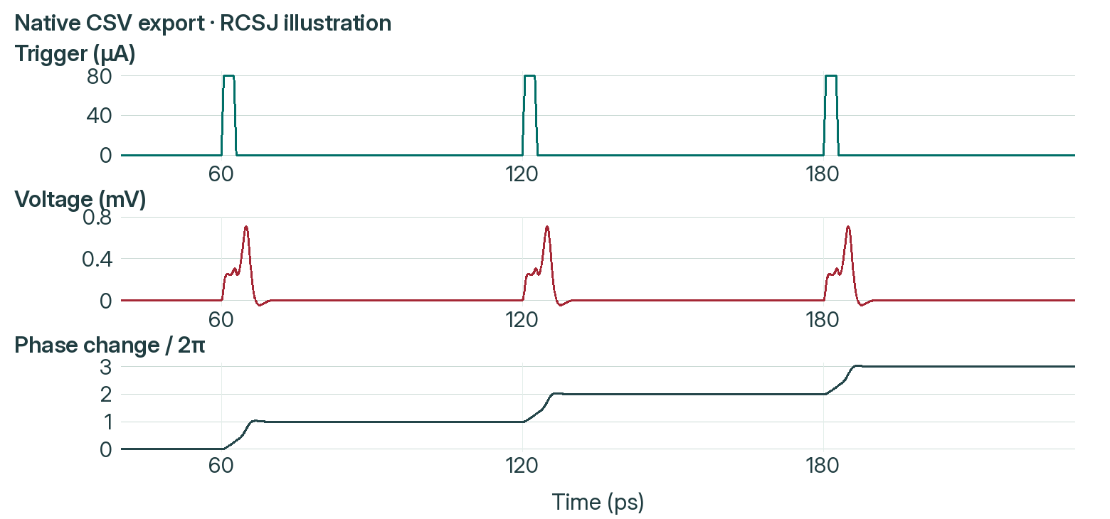
Analysis of the native CSV export, plotted without smoothing or additional samples.
Understanding a single junction phase slip.
The downloadable shunted-junction example contains the .cir input, the native GUI reference CSV and a guide to the model and its interpretation. Use the matching manual and a valid licence to follow the run.
Open the circuit, inspect the schematic and simulate from 0 to 240 ps with a 0.05 ps step. Comparing trigger current, junction voltage and phase shows that each trigger advances the phase by one turn. Integrating the voltage over each settled event gives one flux quantum, consistent with the Josephson voltage relation.
The result was checked against a smaller time step and an independent classical RCSJ reference. It illustrates a generic circuit model, rather than measured device behaviour, a qubit state or a general accuracy benchmark.
Getting started with JoSIM®-Pro.
Documentation and installation
Resources contains the manuals, technical examples and customer download links. Match the documentation and example files to your installed software.
Platforms and licensing
Package families cover Windows x86_64, Linux x86_64 and macOS Apple Silicon. Confirm the supported operating system and architecture with us. Simulation requires a valid JoSIM®-Pro licence and the SUN Magnetics License Manager; evaluation terms and current entitlements are confirmed when discussing your enquiry.
Requesting a quotation
Open Contact, choose “Request a quote”, and select “JoSIM®-Pro” under Product or service. Describe the circuit, intended analysis, platform and automation needs so we can advise on the software and licence.
For a practical starting point, follow the first JTL simulation guide in the knowledge base. It covers the circuit, simulation and result checks for the documented JoSIM®-Pro 2.9 starting path. Check the guide’s version scope against your installation.